I am not sure that there exists a group of bigger SQLite nerds than those of us at Turso.

We use SQLite for everything.. Including for OLAP workloads where we should be using duckdb, or for services which we would love to be totally stateless pods, instead we have statefulsets and PVC's with EBS volumes containing SQLite .db files. Every one of us has probably read just about the entire 265k LOC amalgamation sqlite3.c source file more than once all the way through.

So if anyone has an insight into some of the pain points that will arise from using SQLite in production, surely we are at least good candidates.

But if you ask most Database nerds, what the fundamental limitations are of SQLite, I would guess that almost all will mention at least one of the following:

Exclusive write lock.

The architecture and design around how SQLite manages transaction isolation, as well as their journaling design (which we will cover a bit in #2 as well), means that the writer lock is exclusive and no two connections can obtain a write transaction concurrently. (This is something that tursodb is attempting to fix with MVCC mode.)
Write performance.

At least in WAL mode, SQLite appends all (usually 4kb) pages that are touched as part of a write transaction, referred to as WAL frames, to the log... This includes any and all pages which are shuffled around due to B-Tree balancing, so in theory an INSERT of just a single byte could cause many 4kb pages to be written to the log. Also, when checkpointing (moving these frames from the log to the DB file), SQLite does not use any cached pages it might already have in-memory, it reads each page from disk during the backfilling process and performs N 4kb reads and N 4kb writes where N is the total number of frames needing backfilling. This can cause substantial write amplification and is known to be problematic for write-heavy workloads. For applications which are even moderately write-heavy, which are not gracefully shutting down periodically, typically you have to setup some kind of a background process which monitors the WAL size and periodically forcing a blocking TRUNCATE checkpoint due to the possibility of the WAL growing unbounded.
Checksum/integrity verification.

See this blog post for more details

tl;dr SQLite can 'silently' allow corruption and the user will not find out till much later on.
Read performance for any OLAP style queries.

SQLite’s query engine is extremely good for what it is but its physical join toolbox is intentionally small. By design, SQLite relies on nested loop joins as the core join strategy. That choice keeps the planner simple and predictable, but it comes with some hard ceilings once you push into any analytic-style workloads. This is what we will be talking about today in this blog post.

Join Algorithms: A Brief Tour

Most databases implement a small family of join algorithms:

Nested Loop Join (NLJ):
The simplest: iterate over table A and, for each row, search for matches in table B.
Merge Join:
Requires both inputs to be ordered on the join key. Walk them together like merging two sorted lists.
Hash Join:
Build an in-memory hash table of one input keyed by the join column(s), then probe it with rows from the other input.

There are lots of refinements (index nested loops, block nested loops, hybrid/grace hash joins, etc.), but almost everything is a variant of these.

SQLite fundamentally lives in the NLJ world, making some optimizations.

How Nested Loop Joins Work (and how SQLite makes them fast)

The nested loop join really is as simple as it sounds. The outer loop iterates over one table, and for each row, the inner loop searches the other for matches.

SQLite does add several layers of optimization on top of this:

Using an index on the join column to avoid full scans of table B (so the inner loop becomes an index lookup/Seek rather than a linear scan).
Reordering tables to minimize work
Automatic “ephemeral” indexes when no suitable index exists. SQLite may build a temporary B-tree (we see OpenAutoindex in the plan) to avoid repeated full scans on the inner table.

In SQLite’s VDBE bytecode you can see the basic NLJ shape:

OpenRead cursor for employees

OpenRead cursor for departments

For each row in employees (Rewind/Next loop)

Seek into departments (using persistent or ephemeral index)

Check predicate

Emit result

Oversimplified pseudocode that includes an ephemeral index looks soemthing like:

tempIndex = new BTreeIndex()
for rowA in tableA:
    tempIndex.insert(rowA.key, rowA.RowID)

for rowB in tableB:
    rowID = tempIndex.get(rowB.key)
    if rowID is not None:
        rowA = tableA.seek(rowID)
        output(rowA, rowB)

This works extremely well for small datasets or OLTP-style queries where joins are selective and tables are modest in size. (NOTE: SQLite will sometimes also build a bloom filter as a further optimization, so this can be probed to determine whether or not a Seek should even be done on that join key in the inner loop, but because tursodb does not yet implement this optimization we will pretty much omit this for now)

It also works surprisingly well for a lot of medium-sized workloads, which is why SQLite has done so well with only NLJ.

How can we improve on these optimizations.

For our first improvement, let's consider the following:

SELECT *
FROM large_table_1 AS a
JOIN large_table_2 AS b
ON substr(a.category, 1, 3) = substr(b.category, 1, 3);

Logically this is an equality join, but it’s on expressions rather than raw columns. If there is no index specifically on substr(b.category, 1, 3),

SQLite's query planner has a much harder time constructing an efficient ephemeral index here, so it likely will be a full naive nested loop with scans.

If both tables have million+ rows, it can very quickly turn into tens of billions of comparisons and page touches, even if the page cache saves from reading everything from disk each time.

So overall, ideally we would like to improve on this in two different places:

Use a more performant data structure, to improve on the O(log n) insert/seeks for each outer table row.
Improve the query planner to properly use non 'plain column' expressions as part of our equijoin predicate, and try our best not to fall back to nested scans.

Behold the hash join:

With a similar plan as using an ephemeral index, we can instead use a hash table to get near constant time lookups, at the cost of some additional memory and CPU cycles for hashing.

The general idea is to:

Choose one table as the build input (preferably the smaller one).
Make a single pass over it, building an in-memory hash table keyed by the join column(s).
Then scan the larger probe input, and for each row, do a ~constant-time hash lookup.

If we can choose a hash function that will perform well and avoid collisions as much as possible, we can get fast hashing speed and near O(1) lookups when probing. We can either store the materialized values directly in the hash table, or for more complex/fallback scenarios we can store the rowID of the underlying row, along with the join key (for that case, will cost an additional SeekRowID when a probe matches) and we are able to emit or use the result columns.

The crucial differences vs an ephemeral B-tree:

lookups are ~O(1) instead of O(log N), inserts should be cheaper because they don't require MakeRecord opcode to build the index record with the join key, which in the case of the ephemeral index needs to be saved to compare directly to the probe key, along with the underlying rowid. Also for the common case where we cache the row's payload, we are also saving the additional BTree seek required to fetch the result columns from the row itself, we can store them during the build phase and get the purely constant time lookup.

the hash table is structurally more amenable to optimizations:

partitioning
spilling individual partitions to disk(grace/hybrid hash join)
eventually things like parallelizing build/probe, vectorizing probes, etc.

We think we could improve on the default SQLite features by adding hash joins to tursodb.

Implementing Hash joins in tursodb

Because SQLite (and so of course, tursodb) is implemented as essentially a virtual machine with a storage engine attached, and query plans are just emitted bytecode, adding a new join algorithm will need to consist of creating new Opcodes which we emit at plan time and will be stepped through at runtime and executed by the VDBE (Virtual database engine).

So we are going to need Opcodes to:

HashBuild - feed a build-side row into the hash table.
HashBuildFinalize - finalize the build, potentially spilling partitions.
HashProbe - hash and probe a key, yielding the build-side rowid(s).
HashNext - iterate through additional matches in the same bucket.
HashClose - free the hash table.

Instead of simply using a different data structure for the join, we will also make an attempt to improve the optimizer/query planner.

Remember the example query:

select users.first_name, products.id from users 
join products ON substr(users.first_name,1,2) = substr(products.name, 1,2);

Because neither side of the binary equality expression is a plain Column, and in this case both are expressions, the ast looks something like:
BinaryExpression{lhs: Expr::Function, operator: Operator::Eq, rhs: Expr::Function}

We know SQLite actually will not build an ephemeral index for this query, instead it will fall back to the most naive nested loop join with a full O(n * m) scan. We will improve on this by walking the expressions and tracking the indices into them for each expression that matches the `build` and `probe` tables, this way we can determine that for the following:

pub struct HashJoinOp {
    /// Index of the build table in the join order
    pub build_table_idx: usize,
    /// Index of the probe table in the join order
    pub probe_table_idx: usize,
    /// Join key references, each entry points to an equality condition in the [WhereTerm]
    /// and indicates which side of the equality belongs to the build table.
    pub join_keys: Vec<HashJoinKey>,
    /// Memory budget for hash table (used for cost based optimizations)
    pub mem_budget: usize,
}

pub struct HashJoinKey {
    /// Index into the predicate array
    pub where_clause_idx: usize,
    /// Which side of the binary equality expression belongs to the build table.
    /// The other side implicitly belongs to the probe table, because we will only
    /// ever select equijoin conditions for hash joins.
    pub build_side: BinaryExprSide,
}

The expression will look something like this:

ast::BinaryExpression{ 
    lhs: Expr::Function{func: Func::Substr, args: [ast::Column{users.first_name, ..}, ..], 
    operator: Operator::Eq, 
    rhs: Expr::Function{func: Func::Substr, args: [ast::Column{products.name}..}] }
}

We would walk the ast::Expr, and track that build_side has BinaryExprSide::Left since we are going to use users as the build table, then given the predicate we will be able to translate the expression itself and load the value from the output register directly into the hash table, so the resulting value is hashed and the probe side expression can be compared against it.

Otherwise, we would simply be calling emit_column_or_rowid directly, and instead tracking the column index.. Here we are tracking the expr index and calling translate_expr into the resulting register.

-- simplified
addr  opcode             p1    p2    p3  p4        p5  comment
----  -----------------  ----  ----  --  --------- --  -------
1     OpenRead           0     2     0             0   table=users, root=2, iDb=0
2     OpenRead           1     3     0             0   table=products, root=3, iDb=0
3     Rewind             0     8     0             0   Rewind table users
4       Column           0     1     5             0   r[5]=users.first_name
5       Function         0     5     4   substr    0   r[4]=func(r[5..7]) -- evaluate the function with the col argument -> HashBuild
6       HashBuild        0     4     1             0   
7     Next               0     4     0             0   
8     HashBuildFinalize  3     0     0             0   
9     Rewind             1     20    0             0   Rewind table products
10      Column           1     1     9             0   r[9]=products.name
11      Function         0     9     8   substr    0   r[8]=func(r[9..11])
12      HashProbe        3     8     1   r[12]=19  0   
13      SeekRowid        0     12    19            0   if (r[12]!=cursor 0 for table users.rowid) goto 19
14      Column           0     1     1             0   r[1]=users.first_name
15      RowId            1     2     0             0   r[2]=products.rowid
16      ResultRow        1     2     0             0   output=r[1..2]
17      HashNext         3     12    19            0   
18      Goto             0     13    0             0   
19    Next               1     10    0             0   
20    HashClose          3     0     0             0   
21    Halt               0     0     0             0

The fun part is of course inside HashBuild / HashBuildFinalize / HashProbe: the hash table implementation and how we make it safe for large joins.

Which hash function should we use?

After asking on X, I received some great suggestions from DB veterans, such as XXHash (@_Felipe), and GxHash or rapidhash (@AlexMillerDB) and went down the smhasher rabbit hole, which is pretty much a one stop shop for comparing hash functions.

After a couple of naive benchmarks, I went with rapidhash for the MVP. In the future we may choose different hash functions depending on the key type and size, but “one good, fast hash” gets us very far.

We also fold SQLite-style collations into the hash:

For COLLATE NOCASE text, we hash the to_lowercase() representation.

For COLLATE RTRIM, we trim trailing whitespace before hashing.

For BINARY we hash the raw bytes.

That way equality and hashing line up with the comparison rules the rest of the engine uses.

Spillin’: making hash joins behave under memory pressure (the hard part).

Hash tables are obviously very fast but they can also be incredibly memory-hungry. In a traditional RDBMS, the hash table lives inside the same buffer manager that already knows how to spill to disk and re-read pages. Because SQLite doesn't include the hash table in their toolbox, for tursodb, the hash join is an extra piece of machinery, outside of the pager; so it would be very easy to accidentally blow through RAM on a big join if everything is naively kept in memory.

pub struct HashTable {
    /// The hash buckets (used when not spilled).
    buckets: Vec<HashBucket>,
    /// Number of entries in the table.
    num_entries: usize,
    /// Current memory usage in bytes.
    mem_used: usize,
    /// Memory budget in bytes.
    mem_budget: usize,
    /// Number of join keys.
    num_keys: usize,
    /// Collation sequences for each join key.
    collations: Vec<CollationSeq>,
    /// Current state of the hash table.
    state: HashTableState,
    /// IO object for disk operations.
    io: Arc<dyn IO>,
    /// Current probe position bucket index.
    probe_bucket_idx: usize,
    /// Current probe entry index within bucket.
    probe_entry_idx: usize,
    /// Cached hash of current probe keys to avoid recomputing
    current_probe_hash: Option<u64>,
    /// Current probe key values being searched.
    current_probe_keys: Option<Vec<Value>>,
    spill_state: Option<SpillState>,
    /// Index of current spilled partition being probed
    current_spill_partition_idx: usize,
}
pub struct HashEntry {
    pub hash: u64,
    pub key_values: Vec<Value>,
    pub rowid: i64,
    /// For most cases, to avoid an additional SeekRowID/btree seek on a match, we can
    /// pre-cache the needed result columns in the hash table directly.
    pub payload_values: Vec<Value>,
}
#[derive(Debug, Clone)]
pub struct HashBucket {
    entries: Vec<HashEntry>,
    // ...
}

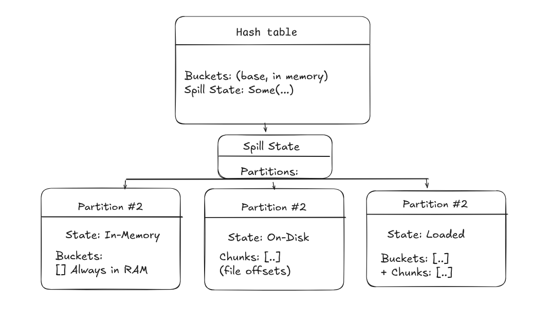
The hash table tracks:

mem_used: approximate bytes for all resident entries in memory.

mem_budget: a soft per-join limit (eventually will be configurable, but will start with 64 MiB by default in release builds).

state: Building, Probing, Spilled, Closed.

During the build phase:

We insert entries and increment mem_used by entry.size_bytes().

If mem_used + entry_size would exceed mem_budget, we:

Initialize a SpillState (if this is the first overflow).
Redistribute existing buckets into NUM_PARTITIONS in-memory partition buffers using the hash value.
Mark the table as Spilled.
Pick one or more partition buffers to spill entirely to disk, freeing their memory.

The spill path uses a very simple on-disk layout:

Each partition has one or more SpillChunk{file_offset, size_bytes, num_entries}.

Each entry is serialized as:

[hash:8][rowid:8][num_keys:varint][key1_type:1][key1_len:varint][key1_data]...

We append a length-prefixed entry blob for each HashEntry in that partition.

After writing a partition:

That partition’s buffer is cleared.
mem_used is reduced by the buffer’s mem_used.
We remember the chunk metadata inside SpilledPartition.

At the end of the build phase, finalize_build does one more pass:

For partitions that have already spilled, any remaining entries are serialized and appended as new chunks.

For partitions that never spilled, we keep them purely in memory:

We consume their PartitionBuffer, build buckets, and mark them as PartitionState::InMemory.
- These are always resident and only counted in mem_used (no disk chunks, no LRU).

At that point we transition to Probing and the build side is “frozen”.

Hybrid Grace hash join and partition reloading.

This algorithm behaves like a hybrid grace hash join, in that we do not hash/partition both the build + probe tables. We attempt to do the whole thing in memory, but if we do spill, than we begin to partition the table and spill only the necessary partitions to disk.

Any partitions that we did have the memory budget for during build time are kept memory resident throughout the entire join and only partitions which did spill are cycled to and from disk and tracked via LRU. We treat the mem_limit for the table as a soft limit and simply try to avoid both drastically exceeding this limit, and thrashing of parititons to/from disk.

Overview

The hash function also determinus a partition index:

fn partition_from_hash(hash: u64) -> usize {
    ((hash >> (64 - PARTITION_BITS)) as usize) & (NUM_PARTITIONS - 1)
}

For partitions that never spilled (PartitionState::InMemory):

There’s nothing special to do; they live in RAM for the lifetime of the join.

For partitions that did spill:

We only load them on demand when the probe hits that partition.

Loading is done via a re-entrant load_spilled_partition(partition_idx):

If the partition is OnDisk, we:

Schedule asynchronous reads for each SpillChunk (we use our own I/O model with hand-rolled state machines and event loop, no async/await).
Accumulate all bytes into a read_buffer.
Once all chunks are read, we parse them into HashEntrys and build buckets.
We estimate the resident memory of those buckets and update accounting.

If the partition is already Loaded, we simply mark it as recently-used in an LRU.

If reads are still in flight, we return an IOResult::IO and the VM yields.

Keeping probe-time memory under control (and avoiding thrash)

pub fn probe_partition(
    &mut self,
    partition_idx: usize,
    probe_keys: &[Value],
) -> Option<&HashEntry> {
    let hash = hash_join_key(...);
    let partition = spill_state.find_partition(partition_idx)?;
    if !partition.is_loaded() { return None; }

    let bucket_idx = (hash as usize) % partition.buckets.len();
    let bucket = &partition.buckets[bucket_idx];
    // scan bucket entries, compare keys, emit matches
}

If we stopped here, probe-time behavior could still be ugly. Imagine the probe side alternates between two “cold” partitions:

We would repeatedly load partition A, then evict it and load B, then evict it and load A again, etc.

To keep things sane, the hash table maintains a small, in-memory LRU cache of loaded spilled partitions:

loaded_partitions_lru: VecDeque<usize> partition indices in LRU order.

loaded_partitions_mem: usize approximate memory used by the loaded spilled partitions’ buckets.

Important distinctions:

mem_used tracks the base in-memory footprint:

The original non-spilled buckets.

Any never-spilled partitions that were materialized in memory.

loaded_partitions_mem tracks only the additional cost of bringing spilled partitions back into RAM.

When we load or parse a spilled partition, we estimate:

fn partition_bucket_mem(buckets: &[HashBucket]) -> usize {
    buckets.iter().map(|b| b.size_bytes()).sum()
}

And before committing to keeping it resident, we call:

evict_partitions_to_fit(resident_mem, protect_idx)

which:

While mem_used + loaded_partitions_mem + incoming_mem > mem_budget:
Picks the least-recently-used partition that is Loaded, and has backing spill chunks (!chunks.is_empty()).
Clears its buckets, resets it to OnDisk, and subtracts its resident_mem from loaded_partitions_mem.

Then we record the new resident partition:

record_partition_resident(partition_idx, resident_mem);

which swaps in the new resident_mem value for that partition + adjusts loaded_partitions_mem and moves the partition to the back of the LRU as most-recently-used.

The effect in practice:

The hash join respects mem_budget during build (by spilling whole partitions).

During probe, it keeps at most a small working set of spilled partitions resident at once.

Typical workloads where only a few partitions are hot see greatly reduced thrash: once a partition is in the LRU, repeated probes for that partition reuse the same buckets.

Pathological workloads where the probe touches more distinct partitions than fit in memory still work; they just spill/reload more often, but at least not entirely arbitrarily/uncontrolled. Eventually if necessary, we can improve on this algorithm further down the road, but when we have more metadata avialable and we are tracking things like total size of each table, that will allow us to make better choices in the query planner, as even choosing the proper table for the build side makes a tremendous difference in performance, as we could avoid spilling to disk entirely in many situations.

When does the planner pick a hash join?

Right now, tursodb is conservative:

We only consider hash joins for queries where SQLite would otherwise build an ephemeral index on the inner side of a nested loop.

We avoid hash joins when a good persistent index already exists and can be used directly, using a real index is always cheaper than building a hash table.

The planner will restrict choosing hashjoins only for INNER equijoins.

We must identify which side should be the build side (this is tough at the moment because we don't track metadata about the size of tables).

Then we generate bytecode that materializes the build input by creating a loop of Rewind/HashBuild/Next for the build table, with any predicates needed from the WHERE clause which might limit the amount of necessary rows needed to hash. (e.g. SELECT t.a, t2.b FROM t JOIN t2 ON t2.c = t.c WHERE t.a > 100, we only have to hash the join keys for rows in t where a > 100), only if the build table is the only table reference in that particular predicate so we can mark it consumed.

Final outcome:

At the risk of this blog post getting far too long, let's look at the best case scenario with our improvements we have made:

Query:

SELECT users.first_name, products.id FROM users 
JOIN products ON substr(users.first_name,1,2) = substr(products.name, 1,2);

No indexes
15k rows per table

Times:
SQLite: 22.772 seconds -- nested loop
tursodb: 2.334 seconds -- hash join

Because SQLite doesn't create an ephemeral btree index here, we are able to get 10x speedup on this query (and we would likely have been able to get similar speedup by just improving the planner and choosing to still build btree index with two expressions).

And a much more fair comparison:

Query:

select users.first_name, products.name from users 
join products on products.name = users.first_name;

No indexes
15k rows per table

Times: SQLite: 20ms -- ephemeral index
tursodb: 15ms -- hash join

You can check out the PR here

Thanks for reading! If you are interested or a fellow database/systems nerd, stop by the repo or the discord, and join our open source community.

Rewriting SQLite: Adding a new join algorithm

I am not sure that there exists a group of bigger SQLite nerds than those of us at Turso.

Join Algorithms: A Brief Tour

How Nested Loop Joins Work (and how SQLite makes them fast)

How can we improve on these optimizations.

Behold the hash join:

Implementing Hash joins in tursodb

Which hash function should we use?

Spillin’: making hash joins behave under memory pressure (the hard part).

Hybrid Grace hash join and partition reloading.

Keeping probe-time memory under control (and avoiding thrash)

When does the planner pick a hash join?

Final outcome:

Query:

Query: